Sentiment Analysis on News Data Using Machine Learning
Sentiment Analysis on News Data Using Machine Learning
- Table of Contents
Goal
Last winter, as part of the Manjum project, I worked on a valuation project using news data. The idea was to crawl news articles about companies, then compare the volume of positive versus negative coverage. The broader goal was to classify articles according to the kSDG (Korea Sustainable Development Goals) framework and automate the assessment of a given company's value and its positive/negative conduct. This post walks through how to crawl news article body text and build a machine learning model to classify sentiment.
Approach
This post assumes the reader has a working knowledge of Python and a basic background in machine learning.
Tools Used
- Python 3.7.5
- konlpy
- keras
- asyncio
- Code used for crawling and machine learning
Crawling
Fast crawling was achieved using asyncio, the asynchronous library bundled with Python 3.7 and later. The news data platform BigKinds provides search results for news data, but it does not support full-body search, so I crawled the content directly. After crawling, many of the parsed data records turned out to be inconsistent with expectations, which occasionally caused the database to crash and caused considerable headaches.
- Some rows had keywords exceeding 5,000 bytes
- Some rows had a null publication timestamp
- Numerous other rows with null values or otherwise malformed data
Once the parsing logic was solid, I introduced asyncio to request and parse pages asynchronously, which made the crawling dramatically faster.
Morphological Analysis
I used konlpy, a Python library for Korean morphological analysis. It works very well aside from neologisms, and the noun dictionary can be customized. The Okt tagger was used.
# Stopwords
stopwords=['의','가','이','은','들','는','좀','잘','걍','과','도','를','으로','자','에','와','한','하다', 'br', '/><', '/>', '.<']

from konlpy.tag import Okt
from konlpy.utils import pprint

okt = Okt()

all_nouns = []
all_nouns2 = []
for row in train_data:
    temp_X = okt.morphs(row[3], stem=True) # Tokenize
    temp_X = [word for word in temp_X if not word in stopwords] # Remove stopwords
    all_nouns.append(temp_X)

for row in test_data:
    temp_X = okt.morphs(row[3], stem=True) # Tokenize
    temp_X = [word for word in temp_X if not word in stopwords] # Remove stopwords
    all_nouns2.append(temp_X)
The library is straightforward to use. Instantiate Okt, then call okt.morphs(string_to_tokenize, stem=True/False) and it returns a string array.
Data Modeling
Morphological analysis turned out to be less difficult than expected. The next step was to transform the text matrices into numpy arrays in a form that a machine learning model can ingest. This also required vectorizing the text — assigning integer indices to tokens rather than passing raw text.
# Tokenize the data
from keras.preprocessing.text import Tokenizer
import json

max_words = 10000
tokenizer = Tokenizer(num_words = max_words)
tokenizer.fit_on_texts(all_nouns)

from datetime import datetime
now = datetime.now()
current_time = now.strftime("%H-%M-%S")
outputfilename = 'all_nouns' + current_time + '.json'

with open(outputfilename, 'w') as outfile:
    json.dump(all_nouns, outfile)

X_train = tokenizer.texts_to_sequences(all_nouns)
X_test = tokenizer.texts_to_sequences(all_nouns2)

print("Max article length: ", max(len(l) for l in X_train))
print("Mean article length: ", sum(map(len, X_train))/ len(X_train))

# Plot the distribution
import matplotlib.pyplot as plt
plt.hist([len(s) for s in X_train], bins=50)
plt.xlabel('length of Data')
plt.ylabel('number of Data')
plt.show()

# Split into training and test labels
import numpy as np
y_train = []
y_test = []

type_of_result = 18
y_result = []
for i in range(type_of_result):
    temp = []
    for j in range(type_of_result):
        if j == i:
            temp.append(1)
        else:
            temp.append(0)
    y_result.append(temp.copy())

for i in range(len(train_data)):
    for type in range(type_of_result):
        if train_data[i][4] == type:
            y_train.append(y_result[type].copy())

for i in range(len(test_data)):
    for type in range(type_of_result):
        if test_data[i][4] == type:
            y_test.append(y_result[type].copy())

y_train = np.array(y_train)
y_test = np.array(y_test)
Machine Learning
This is the step that has the greatest impact on final accuracy.
- Limit total token count with
max_len(e.g. 300) - Choose the embedding dimensionality (e.g. 60)
- Choose the number of LSTM layers (e.g. 30)
- Choose the optimizer and loss function (e.g.
'adam','categorical_crossentropy') - Choose the number of training epochs (e.g. 10)
Full documentation for keras.models is available at the Keras API reference.
from keras.layers import Embedding, Dense, LSTM
from keras.models import Sequential
from keras.preprocessing.sequence import pad_sequences
max_len = 300 # Pad/truncate all sequences to length 300
X_train = pad_sequences(X_train, maxlen=max_len)
X_test = pad_sequences(X_test, maxlen=max_len)

model = Sequential()
model.add(Embedding(max_words, 60))
model.add(LSTM(30))
model.add(Dense(type_of_result, activation='softmax'))
model.compile(optimizer='adam', loss='categorical_crossentropy', metrics=['accuracy'])
history = model.fit(X_train, y_train, epochs=10, batch_size=10, validation_split=0.1)
model.save('lstm_model_yn_'+ current_time + '.h5')
Results
Crawling Speed
- 180 requests, 2700 ms; 1 request: 15 ms
- 9,380 requests, 84,000 ms; 1 request: 9 ms
- 17,036 requests, 201,449 ms; 1 request: 12 ms
The crawling stack was Python + asyncio + BeautifulSoup.
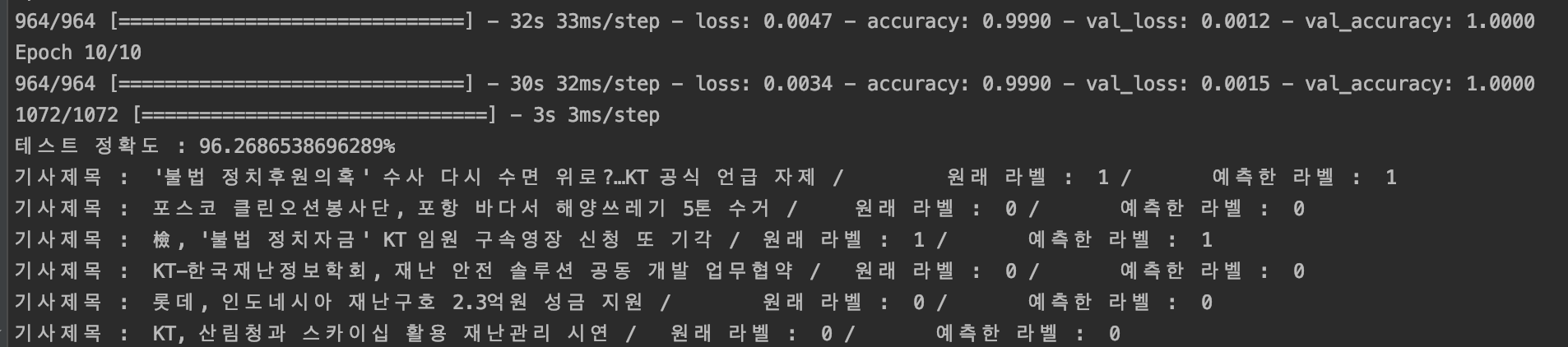
Sentiment Analysis
res = model.evaluate(X_test, y_test)
print(f"Test accuracy: {res[1] * 100}%")

# Compare predicted vs. actual labels
predict = model.predict(X_test)
import numpy as np
predict_labels = np.argmax(predict, axis=1)
original_labels = np.argmax(y_test, axis=1)
for i in range(50):
    print("Article title: ", test_data[i][2], "/\t Actual label: ", original_labels[i], "/\t Predicted label: ", predict_labels[i])
- Accuracy varies with
max_lenper article — longer sequences yield better accuracy but slower inference. - The embedding dimensionality and number of LSTM layers have a significant effect on model size. I tuned these to keep the model within the memory budget for GCP or Heroku (300 MB). Increasing dimensions and layers improves accuracy, but simply scaling them up with a fixed, limited input does not guarantee improvement — it can instead cause overfitting and produce worse results.
- Around 10 epochs tended to give the best outcome. Too few or too many epochs both degraded accuracy.
The sentiment classification results were excellent — 96% accuracy on the evaluation set. I had read that LSTM performs well for sentiment tasks, but I did not expect results this strong. At this level of accuracy, automatically determining whether a given article carries a positive or negative tone is clearly viable as a pre-processing step before valuation. Anyone who needs to solve a sentiment classification problem on raw article text is strongly encouraged to try an LSTM model.
References
- Introduction to Natural Language Processing with Deep Learning — Reuters News Classification
- Deep Learning with Keras
Next
The next post covers deploying the trained machine learning model to the cloud (GAE + Heroku).